Verilog XL Simulation
Overview
In this tutorial you will simulate your 4:1 multiplexor from the previous tutorial. You'll need to remember most of the steps from the 2:1 mux simulation tutorial.
Preparing for Simulation
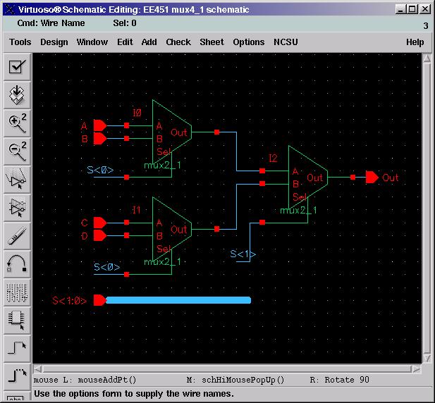
Open the 4:1 multiplexor schematic you created in the previous tutorial. Do this by launching icfb, clicking on your library in the Library Manager, clicking on the 4:1 mux cell and double clicking the schematic view. The schematic window should open up with your mux displayed in it.
Simulation, 4:1 Multiplexor
Cadence offers numerous simulation techniques. For now, we're just going to do a digital behavioral simulation to make sure the multiplexor is logically correct.
In the schematic composer window select Tools -> Simulation -> Verilog-XL. The Setup Environment form will open up. It is automatically filled out based on the schematic window you used to open Verilog-XL so you should already see your library, mux4_1 and schematic in the appropriate boxes. If you don't, use the library browser button to find your mux4_1 schematic.
Press OK. The Verilog-XL Integration form opens up. The next step in your simulation is to write a simulation file. Cadence automatically creates a template file for you, but you need to fill in the guts. Here are the steps to get to the template file:
Select Stimulus -> Verilog...
Agree to creating a test fixture for your design by pressing Yes on the dialog box
This opens the Stimulus Options form.
Change the mode to Copy by pressing the appropriate radio button. Select testfixture.verilog from the scrollbox under file name. Select Make Current Test Fixture and Check Verilog Syntax at the bottom of the form. All the other information defaults to correct values.
Press Apply to make the copy. Notice that the Copy To file name is testfixture.new.
Set the mode to Edit by selecting the correct radio button.
Make sure that file name is testfixture.new.
Press Apply, emacs (or whatever you set your default editor to) should open the testfixture.new file. The text will look like this:
// Verilog stimulus file.
// Please do not create a module in this file.
// Default verilog stimulus.
initial
begin
A = 1'b0;
B = 1'b0;
C = 1'b0;
D = 1'b0;
S[1:0] = 2'b00;
end
Modify the file to simulate your design. Refer to the 2:1 mux simulation tutorial if you need some more help. Here are some ideas for writing more advanced simulation files. They will help you verify every possible input combination.
Bit Concatenation - Remember in the simulation of the 2:1 mux we listed all the inputs on different lines and assigned them one at a time. There is a more efficient way to do this: Bit Concatenation. The 2:1 mux verilog code can be written as:
initial
begin
{A, B, SEL} = 3'b000;
#100;
{A, B, SEL} = 3'b001;
#100;
{A, B, SEL} = 3'b010;
//and so on to test all eight combinations.
end
Other Bases - Using other bases In the initial statement we assign our variables a value. In the bit concatenation example that simulates the 2:1 mux we write the following statment:
{A,B,SEL} = 3'b010;
This means that the concatenated signal {A,B,SEL} is 3 bits wide, thus we need the 3' in our assignment. The b in the assignment says the value will be written in binary. The next 3 digits are the binary value. This should make you wonder if you can use other bases to make assignments, the answer is of course you can. For example, we'll rewrite the above statment using decimal assignment:
{A,B,SEL} = 3'd2;
Notice that we still need the 3' to show that the concatenated singal is three bits wide. Instead of a b we use a d to represent the base is decimal, and then we give the decimal value, in this case 2. If you wanted to write a hex value use a h and then the value. These things will come in handy when simulating a large bus. For example if we had an 8 bit bus and we wanted to set it to have the hex value 0xAA, we would write the following Verilog code.
initial
begin
in[7:0] = 8'hAA;
end
Always list your bus signals as MSB:LSB, this will help you avoid problems with mixing up the MSB and the LSB. The 8' shows the signal is 8 bits wide and the h shows it is a hex number with value AA.
Always and Finish Statements - Another way to simulate the 2:1 mux is to use the always statement. Every always statement needs to have a time and an expression to be executed. For example:
initial
begin
{A,B,SEL} = 3'b000;
end
always #10 A = ~A;
always #20 B = ~B;
always #40 SEL = ~SEL;
always #80 $finish;
Notice the 3 variables need to be initialized in the initial statement. The always statements are after the initial statement. The expressions in the always statements above do the following, after every 10 time segments A will be inverted, after every 20 B inverts and after every 40 SEL. These three statements are executed in parallel which produces the following result:
time | SEL | B | A
0 0 0 0
10 0 0 1
20 0 1 0
30 0 1 1
40 1 0 0
50 1 0 1
60 1 1 0
70 1 1 1
80 $finish
The three always statements have produced exactly the truth table that we wanted. Notice the $finish. This must be included, otherwise the always statements will execute forever.
Simulating Clock Phases - Another wonderful application of the always statement is to simulate the four phases of the clock. In our labs the names of those phases are ph1, nph1, ph2, nph2. You'll learn more about these in class. We want the ph1 and nph1 to always be opposite of each other, ditto for ph2 and nph2. We also want the ph1 and ph2 to always be opposite of each other. The following Verilog code will produce the desired results:
initial
begin
ph1 = 1'b0;
nph1 = 1'b1;
ph2 = 1'b1;
nph2 = 1'b0;
end
always #10 ph1 = ~ph1;
always @(ph1)
begin
ph2 = ~ph1;
nph2 = ~ph2;
nph1 = ~ph1;
end
always #500 $finish;
You'll notice that we initialize all 4 clock phases to be opposite of each other, NOT all to zero as we did in the previous example. The initial statement comes first and then the always statements. The first always statement says every 10 time units ph1 is inverted. The next always statement is read "always at ph1", meaning whenever ph1 changes, do the following things: set ph2 equal to the inverse of ph1, nph2 equal to the inverse of ph2, and nph1 equal to the inverse of ph1. And don't forget the $finish, in this case we will finish our simulation after 500 time units.
After writing and saving the file, close your editor. Set the mode of the Stimulus Options form to Select by clicking on the appropriate radio button. Make sure testfixture.new is selected in filename and press OK. The form should close and you are looking at the Verilog-XL Integration form.
Select Simulation -> Start Interactive or press the upper left hand button on the toolbar. This compiles your testfixture file and gives you some feedback. There should not be any errors or warnings in the command window. If there are, read them and find out what syntax errors you had in your testfixture. Open the testfixture for editing again and fix your mistakes. Try the Start Interactive command again. Repeat this process until you get an error free compile.
Select Simulation -> Continue or press the play button on the toolbar. The simulation completes and displays the output of the $monitor statement in the command window.
You can verify that the 4:1 mux works correctly from just this output, but there is a better way to look at the results. The lower right hand button on the toolbar lets you view waveforms. Press it now. This opens a tool called SimVision. Alternatively you could select Debug -> Utilities -> View Waveform... to open the same window.
SimVision is a waveform viewer. It allows you to view your simulation signals in a graphical format rather than a textual format.
To display the mux simulation waveforms choose Windows -> New Design Browser or click on the toolbar button ![]() . This opens the design browser window from which you will choose which waveforms to display. Expand the test view and click on top. You should now see all the signals in your simulation (A, B, C, D, S0, S1 and Out) in the right hand window. Highlight all of them.
. This opens the design browser window from which you will choose which waveforms to display. Expand the test view and click on top. You should now see all the signals in your simulation (A, B, C, D, S0, S1 and Out) in the right hand window. Highlight all of them.
Right click on the selected signals and choose Send to target Waveform Window or click on ![]() to send the waveforms back to the main SimVision window.
to send the waveforms back to the main SimVision window.
Verify that when S0, S1 are both low, A is reflected at the Output. Verify the rest of the signals as well. Play around with the zoom and fit to screen features so that you are familiar with their use. Fiddle with any other features of the simulator you think might come in handy in the future. The more familiar you are with the simulation environment, the easier future labs will be to complete.
Conclusion
Good job. You have successfully designed and simulated a 4:1 multiplexor. This is the end of the gate level schematic and simulation tutorials.